01 · Hold out a category and search for a map that finds it (UMAP + HDBSCAN) (Search the map space)

Is there a combination of measurements and map settings under which a label nobody showed the map falls out as clusters -- and which unlabelled genes land in them?

Hides one label entirely, walks feature sets and UMAP/HDBSCAN settings, and keeps the map whose clusters best recover that label; unlabelled genes in its pure clusters become candidates, with the shuffled-label score beside them.

Techniques: UMAP, HDBSCAN, Settings walk.
Scorecard (cluster recovery): Weighted F1, Weighted precision, Weighted recall, Adjusted Rand index (ARI), Normalised mutual information (NMI), Homogeneity, Completeness, Unclustered share.

1. Pick the held-out label. Compartment is the classic first question.
2. Leave the grids at their defaults for a first pass (4 maps x 2 cluster sizes x 2 selections); widen n_neighbors to '10, 25, 50, 100' once you know the label is recoverable at all.
3. Set 'Genes per map' to 3000 for speed, 0 for the whole proteome.
4. Press Test first: it hides a quarter of the label, lets the search choose the map and each label's cluster on the rest, and reports how well those clusters hold the hidden genes, against the same clusters scored on the hidden genes with their labels permuted. A FAIL means the chosen clusters hold the label no better than chance.
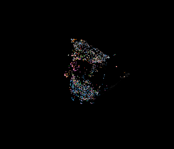
5. Press Run. The best map is drawn, colored by its clusters; 'configurations' ranks every map, 'categories' says which labels were recovered and at what F1.
6. Read 'label clusters' -- the cluster chosen for each label and how well it isolates it -- then 'calls', the unlabelled genes in those clusters. Click a row to find the gene; treat a call's F1 as the most it can be trusted.

How it is tested: 25% of the label is hidden (whole orthogroups together, so no gene is recovered through a visible paralog). The walk is built as set -- its genes per map (up to 4,000), feature sets and grids (up to three values each); the configuration, and the one cluster that best isolates each label, are both chosen using visible labels only. Metric: for each label, the F1 of its hidden genes against its chosen cluster, weighted by size -- does the structure found on known genes hold the unknown ones? Null: the same chosen clusters scored after permuting the hidden genes' labels, 100 times. (A second search on shuffled labels was the null once; it picks the largest cluster for every label, which scores F1 near 2p by size alone and made the null beat real labels.) Pass: above the null's 95th percentile by at least 0.05.

PASS -- F1 of hidden genes in the cluster chosen for their label on known genes 0.132 against 0.039 ± 0.011 under 100 permutations of the hidden genes' labels over the same chosen clusters (bar 0.058, p 0.0099); effect +0.093, needed +0.050; 607 hidden

Hidden: 25% of the compartment labels, whole orthogroups at a time. Null: 100 permutations of the hidden genes' labels over the same chosen clusters.

Scorecard (cluster recovery)

Best of 8 configurations: all permitted, n_neighbors 15, min_dist 0.0, min cluster 20 (leaf). Mean F1 0.271 over the compartment labels, against 0.160 ± 0.006 for the same clustering with the labels shuffled; 2 label(s) recovered at F1 >= 0.5, best 60S ribosome at 0.58. 37 unlabelled genes sit in the cluster that best isolates a label at F1 >= 0.20, and are called with it; 'support' is that F1.