Process images with a point-spread function

Use spacr.point_spread from Python to convolve an image with a point-spread function (PSF), or to deconvolve it with Richardson–Lucy. Prepare a two-dimensional image or three-dimensional volume and a measured PSF sampled at the same pixel or voxel spacing. Supply intensity images; keep object-label masks separate.

Use the desktop controls

In Make Masks, open the enhancement controls and select Convolve (blur) or Deconvolve (Richardson–Lucy) under Point spread function. Enter the image pixel height and width in micrometres. Choose Measured kernel (TIFF/NPY) and load your calibrated two-dimensional PSF, or choose Gaussian approximation and enter the Y/X full widths at half maximum. For a measured kernel, enter its pixel spacing too; it must match the image.

Wait for the kernel to load, then use Compare to inspect its effect. Set Deconvolution iterations when using Richardson–Lucy and choose Apply to use the result for detection. Start with a modest iteration count and inspect noise as well as object boundaries. Reload rereads a kernel file after you change it. Off disables PSF processing.

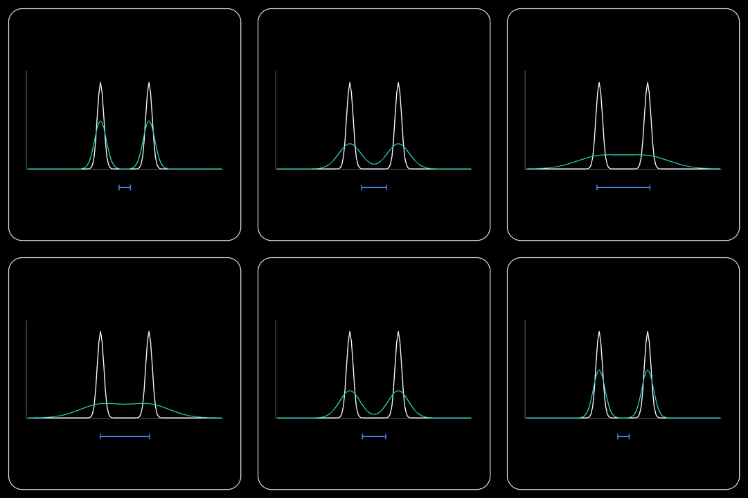
White shows a fixed input profile; teal shows the convolved result. The blue bar indicates the Gaussian kernel’s full width at half maximum. Increasing that width spreads the signal and reduces peak intensity while preserving the integrated intensity. This illustrates convolution with a Gaussian approximation. For your microscope, enter measured calibration values and inspect the resulting image with Compare.

For a batch in Mask or Timelapse, open the Point Spread Function settings category. Set psf_operation to convolve or deconvolve and psf_image_sampling_um to your calibrated [Y, X] pixel spacing. For psf_source="measured", select psf_path and matching psf_kernel_sampling_um. For psf_source="gaussian", supply psf_fwhm_um instead. psf_iterations controls deconvolution work.

Run preprocessing to rebuild the segmentation inputs after changing these settings. One kernel is applied independently to each selected segmentation channel, after illumination correction and before normalization. Check that its calibration is appropriate for all selected channels. The batch operates on two-dimensional projected fields; time-series frames are processed independently. Original image intensities remain unchanged for measurement. Keep psf/segmentation_application.json with the results: it identifies the kernel and processing settings. Reusing existing preprocessing requires an exact completed match. See spacr.psf_pipeline.prepare_psf().

Inspect Mask Live preview

After setting up the PSF, open Live in Mask and choose a representative field. The preview applies the selected kernel before background thresholding and model normalization. Inspect the mask boundaries and processing details, then try another field before running the batch. Raw-intensity object filters continue to use the original intensities.

Live preview normalizes the selected field and does not apply the full pipeline’s illumination correction. A full Mask run may normalize across a batch, so review its saved masks as well as the preview. Changing settings requires a new detection; processing details describe the accepted result.

Choose the intensities used by Measure

In Measure, open Point Spread Function and set psf_measurement_source. Keep original for the standard measurement intensities, including Measure’s normal rescaling and preprocessing, without additional PSF processing. Choose processed to measure intensities after convolution or deconvolution, then configure psf_operation, the kernel source and its calibration.

For a two-dimensional field, enter image sampling and Gaussian widths in [Y, X] order. For a volume, use [Z, Y, X] and a matching three-dimensional kernel. Volume sampling must agree with Measure’s voxel calibration or anisotropy settings. A measured kernel must have the same sampling as the image. Use a kernel appropriate for every selected intensity channel.

Run Measure and inspect the resulting object-feature tables in measurements.db. PSF processing changes the intensity stream used for quantitative features; source files and exported crops retain their usual behavior. The intensity_rescale table records the selected source and PSF processing details. Keep the database with the settings and kernel file.

To compare different kernels or original and processed measurements, use separate projects or output databases. An existing database cannot mix measurements made with different PSF configurations. Restore the recorded configuration when resuming a run. See spacr.psf_measurement.prepare_measurement_psf() for the Python settings contract.

Load the image and PSF

The example below reads a single-channel image and a measured PSF from TIFF files. Replace the example spacing of 0.11 µm with your calibrated Y and X pixel spacing. A three-dimensional input uses Z, Y and X spacing in that order. The PSF must have odd spatial dimensions, a central origin and nonnegative signal after background removal.

import json
from pathlib import Path
import tifffile
from spacr.point_spread import load_psf, apply_psf

spacing = (0.11, 0.11)
image = tifffile.imread("cell_channel.tif")
kernel = load_psf("measured_psf.tif", sampling_um=spacing)

Choose the operation and save the result

Set operation="deconvolve" to perform Richardson–Lucy deconvolution. Start with a modest iteration count and compare the result with the input; more iterations can amplify noise. operation="convolve" instead blurs the image with the PSF. It does not use the iteration count.

result = apply_psf(
    image,
    kernel,
    operation="deconvolve",
    image_sampling_um=spacing,
    iterations=10,
)
tifffile.imwrite("cell_channel_deconvolved.tif", result.image)
Path("cell_channel_deconvolved.json").write_text(
    json.dumps(result.provenance, indent=2), encoding="utf-8"
)

The output preserves the image shape and uses float32 values in the original intensity units. Inspect its range before converting it to an integer image. Keep the JSON record with the result; it contains the kernel identity, sampling and processing settings.

For multichannel images, set channel_axis explicitly: -1 selects a final channel dimension, while 0 selects a first channel dimension. Each intensity channel is processed independently. Image and PSF sampling must match; the function rejects mismatched spacing.

Use a calculated approximation

If your workflow calls for a Gaussian approximation, construct it with spacr.point_spread.gaussian_psf(). Supply the full width at half maximum in micrometres and the image spacing. These are example values to replace with the values appropriate to your analysis:

from spacr.point_spread import gaussian_psf

kernel = gaussian_psf(
    fwhm_um=(0.30, 0.30), sampling_um=spacing, ndim=2
)

Pass this kernel to apply_psf as above. A Gaussian kernel is an approximation; retain that distinction when comparing it with a measured PSF. See spacr.point_spread.apply_psf() for cancellation, progress callbacks and the complete parameter reference.